http://physicstoday.org/journals/doc/PHTOAD-ft/vol_55/iss_3/35_1.shtml?bypassSSO=1
|
articles
The Puzzle of Global Sea-Level RiseMeasuring the rate of sea level rise over the past century requires modeling the behavior of Earth's crust over the past 20 000 years.
Global sea level (GSL) embodies many aspects of the global hydrological cycle and reflects the heat content of the oceans because the density of sea water depends on temperature. GSL is therefore a potent indicator of climate change and a key observational constraint on climate models. GSL is also of immense practical importance. More than 100 million people live within 1 m of the mean sea level. Rising GSL threatens the existence of some island states and deltaic coasts. Coastal wetlands are also endangered because the plants there may be unable to respond to a rate of sea-level rise much beyond what is occurring now, and they will drown if the rate increases substantially. Another threat from rising sea level is the increased erosion of sandy beaches. As a beach is lost, storm waves can more easily reach fixed structures nearby. Those waves will ultimately damage or destroy property unless expensive protective measures are taken. Unfortunately, effective coastal protection is beyond the resources of many developing countries. Compared with those of previous millennia, the changes in GSL occurring today are tiny. Ancient corals found on Barbados reveal that GSL increased by about 120 m as a result of the deglaciation that followed the last glacial maximum of 21 000 years ago. By about 5000-6000 years BP (before present), the melting of the great high-latitude ice masses was essentially completed. Thereafter, GSL rise was small, and appears to have ceased by 3000-4000 y BP. Although the long-term average GSL rise for the past few millennia has been stable at a level near zero, there is reliable evidence from coastal land records,1 lake and river ice cover,2 and water level measurements3 that GSL abruptly began to rise near the mid-19th century. No studies, however, have detected any significant acceleration of GSL rise during the 20th century.4 In the last dozen years, published values of 20th-century GSL rise have ranged from 1.0 to 2.4 mm/y, even though all investigators used essentially the same database of tide-gauge measurements maintained by the Permanent Service for Mean Sea Level (PSMSL) in the UK. In its third assessment report, the Intergovernmental Panel on Climate Change (http://www.ipcc.ch) discusses this lack of consensus at length and is careful not to present a best estimate of 20th-century GSL rise. By design, the panel presents a snapshot of published analyses over the previous decade or so and interprets the broad range of estimates as reflecting the uncertainty of our knowledge of GSL rise. We disagree with the IPCC interpretation. In our view, values much below 2 mm/y are inconsistent with regional observations of sea-level rise and with the continuing physical response of Earth to the most recent episode of deglaciation. This point of contention is not trivial. If the correct value of GSL rise is near 1 mm/y, then global warming provides an appealingly simple explanation: 1 mm/y of GSL rise corresponds to that expected from the thermal expansion of the oceans and the melting of small ice sheets and mountain glaciers caused by the 0.6 °C increase in global surface temperature during the last 100 years. This explanation would further imply that melting of the great Greenland and Antarctic ice sheets is not contributing to GSL rise. But if, as we argue here, the true rate of contemporary GSL rise is closer to 2 mm/y, current climate models will need to be refined. Gauging the tides
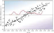
Accurately determining the rate of GSL rise from tide-gauge data is complicated by several issues, the most basic of which is the gauges' poor geographic distribution. Nearly all long and reliable records come from Europe and the US. Furthermore, sea level has enduring low-frequency variations that are coherent over large ocean regions for several decades or more. Figure 1 shows the annual mean relative sea level (RSL) at New York City (NYC) from 1893 to 1995. It also shows RSL for 20-year trends derived by sliding a window over the data set. Clearly, the linear trend result of 2.9 mm/y for the entire 103-year span (black line) represents the overall trend quite well. By contrast, the 20-year trends vary wildly, ranging from 0 to about 6 mm/y. Even 40-year records at NYC have trends that range from 0.9 to 3.5 mm/y. It turns out that RSL everywhere has an interannual-to-interdecadal variation whose amplitude is larger than the underlying rate of rise during a few score years. Consequently, only very long records can accurately yield the underlying trend. This conclusion, derived from tide gauges, is consistent with a new result obtained by Cecile Cabanes, Anny Cazenave, and Christian le Provost of France's National Center for Space Studies (CNES).5 Using in situ measurements of ocean temperature profiles from 1955 to 1996, Cabanes and her colleagues determined regional sea-level trends for the global ocean. To investigate the effect of the geographic distribution of tide-gauge records on estimates of GSL rise, they computed 41-year regional trends at the tide-gauge locations that we had used in some of our studies (reference 6 and chapter 4 in reference 7). The CNES analysis showed that using only four decades of data at the tide-gauge sites led to an overestimate of GSL rise. For a compelling deep-water example of the low-frequency variability of sea level and how it affects the computed trend of sea-level rise, consider Bermuda. The island occupies the top of an extinct volcano and is surrounded by water more than 3 km deep. According to tide-gauge data from 1955 to 1998, RSL rose at Bermuda at a rate of 0.67 mm/y, in good agreement with the value that Cabanes and company calculated for the same interval. But the trend for the entire 1933-98 record is three times larger! In 1990, Dean Roemmich of the University of California, San Diego, computed sea-level heights from a long series of seawater density measurements taken at Bermuda. His analysis showed that the extreme dependence of trend on record length is real, and not an artifact of the tide gauge.8 To remain accurate over periods of a century or more, tide gauges--which over time may be repaired, moved, upgraded, and so on--must be kept consistent. Consistency is maintained by the combination of highly accurate periodic geodetic surveys of the gauge position (usually on a pier) and frequent calibration of the gauge itself. But tide gauges, no matter how accurate and consistent, make local measurements. And they measure only relative sea level with respect to the surface of the solid Earth. Without independent estimates of vertical land movement, tide gauges cannot determine whether the water level is rising, the land is sinking, or both. Altimetric satellites, such as TOPEX/Poseidon (launched in 1992 and still operating) and Jason 1 (launched in December 2001), observe almost the entire planet and determine the absolute, not relative, sea level because they make measurements with respect to Earth's center of mass. The newest satellite mission is GRACE, the Gravity Recovery and Climate Experiment. Scheduled for launch in March 2002, GRACE is based on a paired satellite-satellite tracking system and will measure the time dependence of the planet's gravitational field. GRACE is expected to measure GSL rise with an accuracy of a small fraction of 1 mm/y. Satellite determinations will predominate in the 21st century, but presatellite 20th-century values are still needed to see if the rate of GSL rise has accelerated. Bouncing back
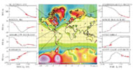
Vertical land movements at tide-gauge sites are a significant contributor to the complexity of determining GSL rise. The effects of plate tectonics eliminate a large number of tide-gauge records from consideration, particularly at colliding plate boundaries. Tide gauges in Alaska, Japan, India, and many other areas have long records that are unusable because of vertical uplift or subsidence associated with seismic activity or crustal deformation.6 Volcanism, sediment compaction, and underground fluid extraction also cause vertical movements that render many tide-gauge sites useless for determining GSL rise. But the most widespread source of vertical land movement is glacial isostatic adjustment (GIA), the gradual springing back of Earth's crust in response to the removal of the ice loads of the last glacial maximum (LGM), which were at their maximum extents around 21 000 y BP. Figure 2 shows the locations of the LGM ice sheets. In magnitude, GIA and RSL rise are comparable over the entire surface of the planet. Determining the response of RSL to the removal of these ice loads depends on Earth's rheology, which, in turn, depends on frequency. At seismic or tidal frequencies, Earth behaves elastically--like a ball of Silly Putty® that bounces when dropped. But at the extremely low frequencies associated with glacial loading and unloading, Earth responds viscoelastically. When the long-enduring LGM ice loads disintegrate, the resulting imbalance of the gravitational force begins to restore the shape of the planet to its previous unglaciated form.
In a recent paper, Glenn Milne of the University of Durham in the UK and his collaborators used the global positioning system (GPS) to measure horizontal and vertical land motions in Fennoscandia.9 The GPS measurements, in combination with a geophysical model, suggested that the falling RSL in Fennoscandia consists of a regionwide increase of sea level at the rate of 2.1 ± 0.3 mm/y, superimposed on individual, larger, site-dependent decreases caused by GIA. The overall regional rate is essentially identical to our own previously published estimates of the globally averaged rate of RSL rise, in which we took into account the influence of GIA on a carefully selected subset of long tide-gauge recordings (reference 6, chapter 4 in reference 7, and reference 10). Milne's approach of using GPS measurements to correct tide-gauge records of RSL change has great potential for determining the rate of GSL rise. But the requirement remains that the RSL records span almost a century. Satellite-borne radar altimeters do not need such long records to determine GSL. With a nine-year baseline, TOPEX/Poseidon currently yields a value for GSL rise of 2.4 mm/y (chapter 6 in reference 7), close to the best values from GIA-corrected tidal gauges. But a few more years of data are required before a value significantly below 2 mm/y can be excluded with a very high level of confidence.
Geology and geophysicsGPS measurements require a decade or more to determine solid Earth uplift or subsidence rates of less than 1 mm/y, the precision needed at midlatitude tide-gauge sites. Other methods have therefore been used to correct historical RSL trends for GIA. These methods adopt either a geological or a geophysical approach. The geological approach involves no physics. Site-specific or regional geological rates of GSL change are deduced from sea-level indicators that date from the Holocene epoch (10 000 y BP to the present). In the geophysical method, theoretical models of global GIA are built that are consistent with geological, astronomical, and other observations and that incorporate the rheology of the solid Earth. Although, in special cases, the geological method may provide an acceptable means of compensating for GIA, the required data are not always available and are susceptible to sometimes severe extrapolation error. By contrast, a comprehensive global geophysical model is now available that can accurately correct both tide-gauge and satellite altimetry-derived measurements for GIA. Developed by one of us (Peltier) and his collaborators at the University of Toronto, the geophysical model describes the gravitational interaction between a spherical viscoelastic model of the solid Earth and the surface mass load (varying in time and space) associated with the process of glaciation and deglaciation.11 The load consists of both ice and water components whose total mass is conserved because Earth's hydrological cycle is essentially closed. Besides this most fundamental constraint, the primary concept underlying the theory is that the meltwater produced as the LGM ice sheets disintegrated must be distributed over the surface of the global ocean in such a way that this physical surface remains one of constant potential. Because the GIA process occurs on a timescale that is long compared with mean circulation effects, we can accurately predict variations in Earth's gravitational potential that GIA causes. In the Toronto model, the viscoelasticity of Earth's mantle is described as a three-dimensional (3D) linear Maxwell solid. When subjected to an instantaneous shear stress, a Maxwell solid responds initially as a Hookean elastic solid but as a Newtonian viscous fluid on time scales longer than the "Maxwell time" of about 200 years. The viscosity that governs the creep of a polycrystalline solid material, such as Earth's iron magnesium silicate mantle, is expected to be a strongly 3D function of position. This expectation arises because the creep of a polycrystal is a thermally activated process and because only a strongly 3D temperature distribution could be responsible for the vigorous thermal convection required to cause the observed continental drift at Earth's surface. Nevertheless, it appears possible to explain observations of the sea-level variations induced by deglaciation with a model in which the variation of viscosity through Earth's mantle is a function of radius only.
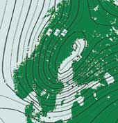
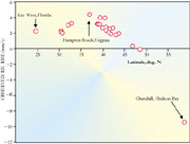
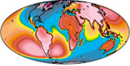
The highly structured nature of the spatial variation of the GIA signal is readily apparent in Figure 4. Strong postglacial rebound (falling RSL) occurs in the deglaciated regions, surrounding which are regions of rising RSL controlled by the collapse of the feature known as the proglacial forebulge. As its name suggests, the proglacial forebulge is a surface deformation of the solid Earth caused by the viscous outflow of material from under the ice-loaded regions. When the ice sheets disintegrate, the unbalanced gravitational force induces a return flow of material that drives crustal rebound in the previously ice-covered region. That same flow simultaneously causes the forebulge to collapse. On the US East Coast, the predicted rates of RSL rise due to forebulge collapse reach or exceed 1 mm/y, the highest rates of GIA-induced RSL rise anywhere in the US. Comparing this rate to the secular rate of RSL rise for NYC shown in Figure 1, it is apparent that approximately 30% of the 20th-century trend of 2.9 mm/y is due to GIA rather than to modern climate change. We therefore infer that modern climate change contributes 2 mm/y to the rise in sea level at NYC. An interesting heuristic approach to determining the rate of GSL rise can be made by examining the 20th century sea level trends for eastern North America. Figure 5 displays the observed RSL trends (that is, uncorrected for GIA) along a geographical swath extending southward from the port of Churchill on Hudson Bay in Canada to Key West off the Florida coast. We obtained the trends from PSMSL and used only records that spanned at least 60 years. During the LGM, a vast ice sheet, centered on what is now Hudson Bay, covered the northern half of North America. The Figure shows that RSL rise tends asymptotically toward a value of 2 mm/y as the distance from Hudson Bay increases and the effect of GIA decreases. Also evident in the Figure is the presence of the proglacial forebulge, which peaks over the Chesapeake Bay. When the RSL data shown in the Figure are corrected for the effect of GIA and averaged along the coast,12 the value of GSL rise obtained that can be attributed to modern climate change is 1.9 mm/y, regardless of whether the GIA correction is determined geologically from Holocene sea-level indicators or geophysically from the tuned global model.
Accurately measuring regional sea-level rise or GSL rise in 1-2 decades requires satellite data, which, like tide-gauge data, require a correction for GIA. This correction is different from the one used for tide gauges because satellites measure sea level with respect to Earth's center of mass, as opposed to the surface of the solid Earth in the case of tide gauges. As a result, if the theory-based model shown in Figure 4 is to be used to correct satellite data, an extra term must be added to the prediction--namely, the predicted rate of radial displacement of Earth's surface with respect to the planet's center of mass.
Solving the puzzleThat our best estimate of the rate of GSL rise for the past century is closer to 2 mm/y than 1 mm/y must be seen as posing a definite geophysical puzzle. In the most comprehensive currently available study of the oceans' heat content, Sydney Levitus of the National Oceanographic and Atmospheric Administration and his colleagues estimate that the thermal expansion of the oceans contributes 0.6 mm/y to GSL rise (see Physics Today, June 2001, page 19*). The melting of small ice sheets and glaciers also contributes to GSL. According to Mark Meier of the University of Colorado, the latest and best upper bound on this contribution appears to be near 0.3 mm/y. Together, these two contributions amount to less than 1 mm/y, leaving a deficit of the same order to be explained. One possible resolution of the puzzle would be a clear demonstration that all the century-scale tide-gauge records used in the analyses that we and others have performed are biased upward--perhaps as a consequence of a strong enhancement of the influence of thermal expansion at coastal locations. This solution has recently been proposed by Cabanes and her colleagues. A second possible solution to our puzzle is that the true global rate of secular GSL rise is indeed closer to 2 mm/y than to 1 mm/y, implying that the great polar ice sheets on Antarctica and Greenland are losing mass at a net rate that contributes 1 mm/y to the global value. A significant impediment to this possibility comes from the constraint on the present-day rate of polar ice-mass loss provided by Earth rotation observations. As demonstrated in several early analyses of the influence of GIA on Earth rotation, both the so-called nontidal acceleration of Earth rotation and the ongoing secular drift of Earth's pole relative to the surface geography are explained well by the same GIA model that explains the RSL data shown in Figure 3.14 Furthermore, the nontidal acceleration of rotation anomaly is so sensitive to the present-day melting of polar ice that, if the best currently available result derived from satellite laser ranging is correct, it would be impossible to solve the puzzle by invoking the required rate of mass loss from Greenland, Antarctica, or both.11 If, however, it could be demonstrated that the laser ranging result was in significant error, this solution would become both possible and attractive. A third possible solution of the puzzle is that Levitus's estimate of the influence of thermal expansion is significantly biased downward as a consequence of undersampling the Southern Hemisphere ocean at all depths and the abyssal ocean in both hemispheres. In our opinion, none of these individual possibilities can be entirely ruled out at present, nor can the possibility that the key may involve a mix of all three. The global measurements to be provided by the imminent GRACE mission and by continuing efforts in satellite altimetry are expected to provide a definitive solution to this important climatological and geophysical puzzle. But several years of data and further efforts at interpretation will doubtless be required.
1. M. S. Kearney, J. C. Stevenson, J. Coastal Res. 7 (2), 403 (1991).
2. J. J. Magnuson et al., Science 289, 1743 (2001).
3. P. L. Woodworth, Geophys. Res. Lett. 26, 1589 (1999).
4. B. C. Douglas, J. Geophys. Res. 7 (c8), 12699 (1992).
5. C. Cabanes, A. Cazenave, C. le Provost, Science 294, 840 (2001).
6. B. C. Douglas, J. Geophys. Res. 96 no. C4, 6981 (1991).
7. B. C. Douglas, M. S. Kearney, S. P. Leatherman, eds. Sea Level Rise: History and Consequences, Academic Press, San Diego, Calif. (2001).
8. D. Roemmich, in Sea-Level Change, National Academy Press, Washington, DC (1990), p. 208. Also available online at http://www.nap.edu/books/0309040396/html.
9. G. A. Milne et al., Science 291, 2381 (2001).
11. W. R. Peltier, Rev. Geophys. 36, 603 (1998).
12. W. R. Peltier, Geophys. Res. Lett. 23, 717 (1996).
13. P. Wu, W. R. Peltier, Geophys. J. R. Astron. Soc. 76, 202 (1984). W. R. Peltier, Global and Planetary Change 20, 93 (1999). J. X. Mitrovica et al., Geophys. J. Int. 147, 562 (2001). W. R. Peltier, Quat. Sci. Rev. 21, 377 (2002).
14. W. R. Peltier, Nature 304, 434 (1983). W. R. Peltier, Science 240, 895 (1988).
|
|